Service Navigation
Search
Weather models map the events in the atmosphere with the help of mathematical formulas. These numerical forecast models are now the standard method of producing weather forecasts. Considerable progress has been made in recent decades in understanding the chemical and physical processes in the atmosphere. Furthermore, the spatial resolution (mesh size) of the numerical models has greatly improved.
How uncertainty arises
Despite the progress that has been made, some processes can still not adequately be represented by numerical models. Some are still represented by means of parameterisation, whereby a process is not represented physically on the basis of one or more physical laws, but in a simplified way using a surrogate method.
Further uncertainty arises when the values of the individual parameters describing the state of the atmosphere at the beginning of the numerical simulation are not definitively known. This is the case in spite of the fact that frequent observations and measurements (e.g. those taken at ground-level weather stations and various observation networks for gathering atmospheric data enable continual improvements to be made.
These values (also called initial conditions) are important for initiating the model simulations. Due to the chaotic nature of the atmosphere, small differences or uncertainties in the initial conditions can lead to large differences between simulations produced by the same numerical forecasting model.
How uncertainty is quantified
Consequently, every weather forecast is subject to a certain degree of uncertainty. To quantify this uncertainty, a so-called ensemble approach is used for the numerical models. This means that several scenarios are calculated for the same time period using the same numerical model, but with slight adjustments, e.g. to the initial conditions that are entered as the starting parameters for the simulations. In contrast, when a single scenario is calculated and represented, this is referred to as a deterministic approach.
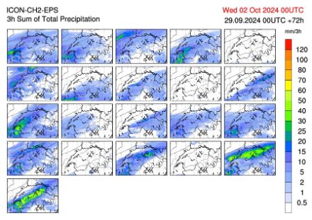
For example, the high-resolution numerical model ICON-CH1-EPS (which uses a horizontal mesh size of 1.0 km) computes 11 scenarios, or “ensemble members”, eight times a day for a forecasting period of up to 33 hours. The ICON-CH2-EPS model, which uses a horizontal mesh size of 2.1 km, predicts 21 scenarios for a 5-day period.
To illustrate the ensemble approach, the figure below shows the forecasts simulated for 21 different ICON-CH2-EPS model scenarios for the predicted 3-hour precipitation total at 9 UTC (Coordinated Universal Time) on 24th July 2020. For this period, covering 27 hours from the start of the simulation, there are clearly large differences between the scenarios. This highlights the uncertainty associated with a forecast of the expected precipitation amounts for that day and their timing. Specifically, depending on the ensemble member considered, either a dry (precipitation-free) or a wet (precipitation-rich) scenario could be forecast for a given point or region.
Integration of probabilistic forecasts
MeteoSwiss has systematically integrated this probabilistic approach into its forecasts and meteorological services. This is seen particularly in weather forecasts, which use a number of probabilistic terms for phenomena associated with a higher degree of uncertainty:
Probabilistic terminology in the weather forecast
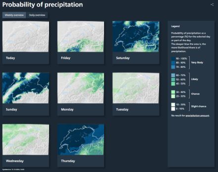
Probabilistic information is also increasingly incorporated into the graphical representations of our forecasts. The Precipitation Probability application shows the probability of precipitation for the next few days in the form of maps. The probability of precipitation is calculated directly from the ensemble forecast: the proportion of scenarios or members with precipitation indicates the probability of precipitation. This representation only provides information on the probability of precipitation, not on the amount of precipitation.
The probability maps are available for whole days (24 hours) and for periods of 6 hours. How should these maps be interpreted and what does a 30% chance of rain mean, for example? It is important to mention that the probability does not indicate the duration or intensity of precipitation. It means that for the chosen time period, 30% of the model members expect precipitation and 70% expect dry weather.
The time interval for which the probability forecasts were generated is also important. The probability of precipitation in 24 hours will always be higher than for a period of 6 hours, because there is more time available in which precipitation could occur.
Care should be taken when interpreting probabilities of precipitation in thunderstorm conditions. In general, the probabilities are lower in such situations than in the case of an extensive precipitation event. This is due to the localised precipitation patterns (thunderstorm cells), which can look very different between the model members.
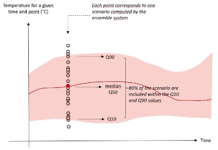
The local forecasts also include probabilistic information. On the basis of the ensemble scenarios, one median scenario can be calculated for each meteorological parameter for a specific place and time. This means that half of the scenarios in the ensemble forecast will return a higher value and the other half a lower value than the median scenario. To quantify the most extreme values predicted by these scenarios, the highest 10 percent of the higher values and the lowest 10 percent of the lower values are used. The value below which the lowest 10 percent lie is called the 10% quantile (Q10), while the value above which the highest 10 percent lie is called the 90% quantile (Q90). (The median is the 50% quantile.)
Probabilistic information on the MeteoSwiss website
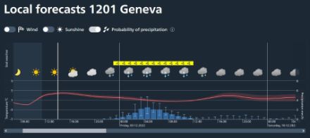
The example of Cabane du Trient CAS shows how probabilistic information is integrated into the local temperature and precipitation forecasts. The median temperature (Q50) is represented by a red curve. The semi-transparent pink uncertainty cloud between quantiles Q10 and Q90 comprises the remaining 80% of the scenarios calculated by the ensemble system. With the ICON-CH2-EPS model, for example, this would mean that about 17 out of 21 available scenarios would fall within this range.
The median precipitation amount is represented by a blue bar. This indicates the expected precipitation amount. The uncertainty range is represented by a light blue vertical line, bounded above and below by horizontal lines corresponding to quantiles Q10 and Q90. As with temperature, 80% of the scenarios calculated by the ensemble system fall within the area between these two quantiles.
Here, too, care should be taken in the case of thunderstorm conditions. If a thunderstorm is forecast for a specific location, the indicated median value is often significantly too low. In the case of thunderstorms, the uncertainty is far greater than in the case of extensive precipitation – and the earlier the forecast is generated, the less accurate the model forecasts and the probabilities derived from them will be.
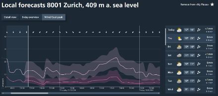
Probabilistic information in the MeteoSwiss App
Probabilistic information is also integrated into the temperature and precipitation forecasts in the MeteoSwiss App.
The information in the app and on the website is identical. It differs only in terms of presentation.
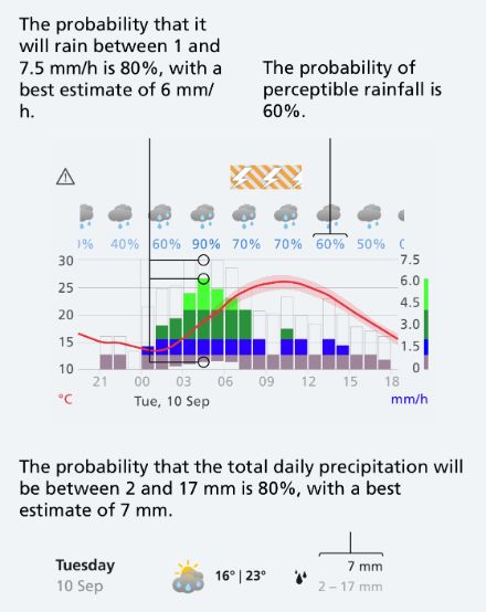
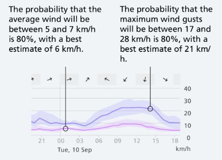
The uncertainty of the temperature and wind forecast is represented by a semi-transparent area. The larger this area is, the greater the uncertainty. The probability that the value falls within this area is 80%.
The uncertainty of the precipitation forecast is displayed in various forms. The transparent columns represent the uncertainty of precipitation intensity. The blue percentages indicate the probability that it will rain perceptibly within 3 hours. The intervals in the weekly overview indicate the uncertainty of the daily precipitation total. Graph showing the expected development of temperature and precipitation, both for the best prediction scenario and using uncertainty ranges.