Service Navigation
Search
Climatological classification of an event
This section presents a typical approach for classifying a precipitation event. We take the example of the flood that affected the village of Lully (Canton of Geneva) on 14 and 15 November 2002. It was caused by heavy precipitation related to the passage of a cold front over Switzerland and to the transport of moist air from the Mediterranean. Knowing whether this event was out of the ordinary and how often similar events could occur in that region may be of interest for improving the canalization system and managing future floods in that region. The web platform “Extreme value analyses” provides useful information to answer these questions.
An essential task for the classification of an event is the definition of the region and the precipitation quantities of interest. Which part of Switzerland was affected? Was the precipitation responsible for the damage of short or long duration?
Identification of the region and station(s) of interest
In a first step, the region of interest (e.g. the zone affected by a flood) and the stations that can be used for the analysis must be identified. Should no station be available in the area, stations located nearby with a comparable climate can be used instead.
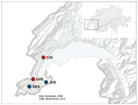
In our example, no MeteoSwiss observation station is located in the village of Lully. The closest MeteoSwiss stations available are Genève-Aire and Genève-Cointrin, which measure respectively daily and hourly precipitation.
Determination of the duration of the event
The second step consists in defining the duration of the event in order to determine the precipitation sums that are relevant for the analysis using all available means (e.g. hyetographs, radar images, etc.). This depends not only on the actual time interval in which the event took place, but may involve a subjective choice, as stations within the MeteoSwiss observational network measure precipitation at fixed times of the day. For example, hourly precipitation is measured from hh:40 to hh:40, while daily precipitation is measured from 05:40 UTC of one day to 05:40 UTC of the following day.
The figure below illustrates the decision that has to be made. It shows the hourly precipitation at station Genève-Cointrin, the station measuring hourly precipitation located closest to the village of Lully, during the event of 14-15 November 2002. At that station, two phases of relatively intense precipitation were measured between 14 November 04:40 UTC and 15 November 03:40 UTC (gray background), while only little precipitation was measured before and after those phases (respectively on 13 and 15 November). It thus makes sense to consider the 1-day precipitation when analyzing this event. However, since the measurement of daily precipitation starts only at 05:40 UTC, by considering the 1-day precipitation of 14 November (green vertical lines), the first hour of precipitation of the event would be excluded here.
In this case, the precipitation event nearly coincides with the time of the measurements and only little precipitation would be left aside by selecting the 1-day precipitation sum. However, it is often not the case and it might be necessary to consider a longer time frame than the actual duration of the event. Examples of such a decision can be found on the High impact precipitation events page, where different precipitation durations were used to analyze the presented events.
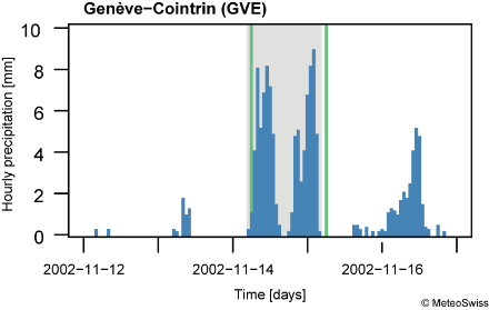
In the figure above, hourly precipitation [mm] is represented by vertical blue bars. The ticks on the time axis mark the beginning (00 UTC) of the days. The gray background shows the duration of the event, while the green vertical lines indicate the beginning and end time of the period over which the 1-day precipitation (for 14 November 2002) is cumulated.
In our example, it makes sense to consider the 1-day precipitation for the analysis, even though this might mean excluding a few hours of precipitation at the beginning of the event. We also assume that since the precipitation during the event extended over a relatively large area over the western part of Switzerland, it followed a similar pattern in the whole region of Geneva. For example, the magnitude of the precipitation measured at the nearby station Genève-Aire is very similar to what was measured at station Genève-Cointrin during the event, as well as before and after the event (see table below). Since these two stations are located only 4-8km away from the village of Lully, one can suppose that the precipitation was not very different in Lully and had similar duration and magnitude.
Daily precipitation [mm] measured between 13 and 15 November 2002. Precipitation sums are measured from 05:40 UTC of one day to 05:40 UTC of the following day. Source: MeteoSwiss
| Station | 13.11.2002 | 14.11.2002 | 15.11.2002 |
|---|---|---|---|
| Genève-Aire | 2.1 | 93.5 | 9.5 |
| Genève-Cointrin | 4.1 | 92.6 | 6 |
Usage of the web platform
Once the relevant stations and precipitation sum(s) have been selected, the web platform can be used to retrieve the return periods of the precipitation amount(s) observed in the selected duration interval(s). Below, we show how to retrieve this information and present further functionalities of the web platform (click on one of the topics to expand the information box).
Here we chose to show only station Genève-Aire, which is the station located the closest to the village of Lully. Obviously, the same operation should be repeated for all the stations in the region of interest, in order to find the best station for the estimation of the return period of a given event
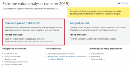
The standard period should be used for the climatological classification of an event. It can be selected on the entrance page.
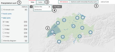
- o select the relevant precipitation sum(s), click on the appropriate checkbox(es) (1).
- To select a station on the map, click on the number in the region in which the station of interest is located (2); it will zoom in. You might have to click several times until the the name of the station is displayed. Then, click on the station in order to view the extreme value analysis page. Note that if the name of the station is known (correct orthography in local language), it can either be accessed by selecting it in the table listing all the stations (3) or by entering its name in the top left corner of the map (4).
Alternatively, select the station first and afterwards the precipitation sum(s). Note that a filter can be applied to display only stations with sub-daily measurements (5). By default all stations are displayed.
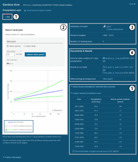
Clicking on a station opens a blue box; this is the extreme value analysis page, which displays the extreme value analyses for the precipitation sums chosen. The following information are found on this page:
1) Tabs with the selected precipitation sum(s)
The sum currently displayed is indicated by a red line at the top of the tab (in this case 1 day).
2) Return level plot and data query
The return level plot displays the return levels and their uncertainty (ordinate) for a given return period (abscissa) for the selected precipitation sum. The return level estimates are given by the blue line, while their 95% confidence bounds are colored in green. By default the 95% confidence bounds are displayed, but the 68% confidence bounds can also be selected (blue box).
The data query for return levels or return periods (gray box) can be used as follows:
- Return period query: click on “return period” (if not already active) and enter a precipitation amount in the query field. A grey horizontal dashed line appears at the height of the precipitation amount (return level) on the return level plot. Simultaneously, the corresponding return period is retrieved and appears with a vertical dotted line. For example in the figure below, the query for a return level of 93 mm/day gives a return period of 80 years.
- Return level query: click on “return level”, then enter a length of time in years in the query field (e.g. 35 years). A grey vertical dotted line appears for the return period and a grey horizontal dashed line appears at the height of the estimated return level. A green shaded area also indicates the uncertainty of the estimation.
3) Information about the results and underlying data
Please note that particular attention should be given to the reliability of the results and that the methodological information should be consulted before using the analyses.
4) Documents to download
These include the extreme value analysis, the results of the analysis in CSV files, as well as a link to the user manual and documentation (methodological background).
5) Tables of the estimated return levels for selected return periods and of the return periods of the 10 largest annual sums
These tables can also be downloaded as CSV files.
With the help of the web platform, we have determined that, based on the analysis at station Genève-Aire, the event of 14-15 November 2002 that caused floods in the village of Lully could have been rare. Since this station is located only 4km away from the village of Lully and since the precipitation extended over a relatively large part of western Switzerland, we can assume that the precipitation had comparable duration and magnitude in Lully as at station Genève-Aire. That day, 93.5 mm were measured at that station, which corresponds to a return period of around 80 years. This should be taken into account in the design of future flood managing measures.